Date Filter in Pivot Table
A date filter in pivot table allows you to filter data based on date criteria. This is especially useful when you have a large dataset with date-related information and you want to focus or analysis on specific date ranges or periods.
Contents
ToggleLet’s discuss some important Date filters here:
- Individual Date with the Date Check box (Report filters only have this type of date filter)
- Selection by specific Date Range
- Dynamic Date Range or Date Grouping
- Custom Filter
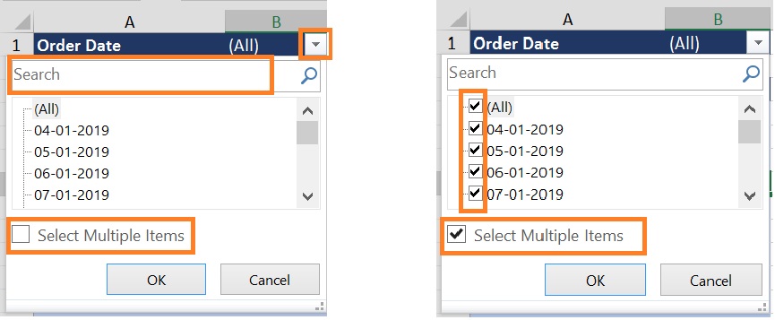
Individual Date with the Date Check box
If a date field is in the Report Filter area, only the date check boxes are available.
- Click the drop-down arrow on the date field
- Add a check-mark to “Select Multiple Items” to show the check-boxes.
Otherwise, only the list of dates will show and you will able to choose one at a time - In the list of dates, add check marks to show dates and uncheck to hide specific dates.
- Then click OK
Selection by specific Date Range
This filter is only available in the Row or Column Labels filter, when the date field is placed in the Row or Column area in the pivot table fields.
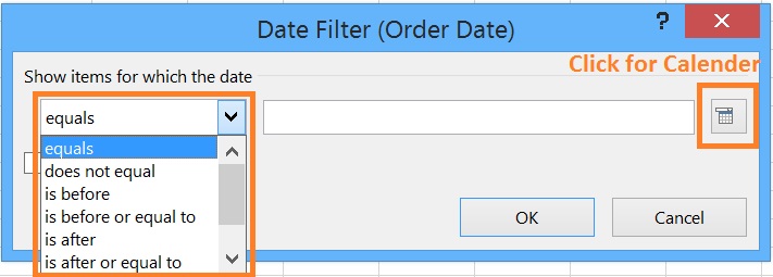
This filter includes Equal, Before, After, and Between – You can specify a specific date by directly entering or selecting from the calendar that is available there. This is useful for analyzing data within a particular time frame. A dialog box will appear for custom filters.
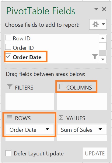
Add Date Field to Rows or Columns:
- Drag and drop the date field you want to filter into the Column Labels or Row Labels area of the Pivot field section.
Filtering by Date:
- Click the down arrow next to Column Labels or Row Labels in the Pivot Table
- Then you will see “Date Filters” so Select Date Filter Type from the list.

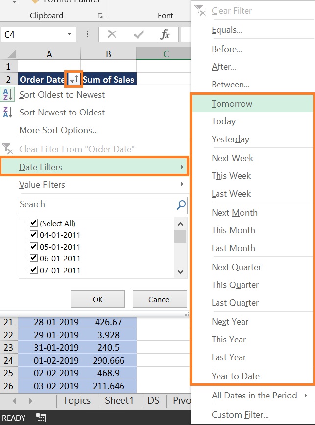
Dynamic Date Range or Date Grouping
This filter is also only available in the Row or Column Labels filter, when the date field is placed in the Row or Column area in the pivot table fields.
A dynamic range changes automatically based on the current date. For example, Tomorrow and Yesterday represent a day after today and a day before today respectively, and will change automatically every day when you open the pivot table file.
Apply Dynamic Date Range Filter:
- Drag and drop the Date field you want to filter into the Column Labels or Row Labels area of the Pivot field section.
- Click the down arrow next to Column Labels or Row Labels in the Pivot Table.
- Then you will see “Date Filters”
- Then select Date Filter Type from the list.
Dynamic date range options are the following:
- Single Day: Tomorrow, Today, Yesterday
- Single Week: Next Week, This Week, Last Week
- Single Month: Next Month, This Month, Last Month
- Single Quarter: Next Quarter, This Quarter, Last Quarter
- Single Year: Next Year, This Year, Last Year
- Year to Date
Other Dynamic date range options are also available:
- Every Quarter: Quarter 1, Quarter 2, Quarter 3, Quarter 4
- Every Month: January, February……………December
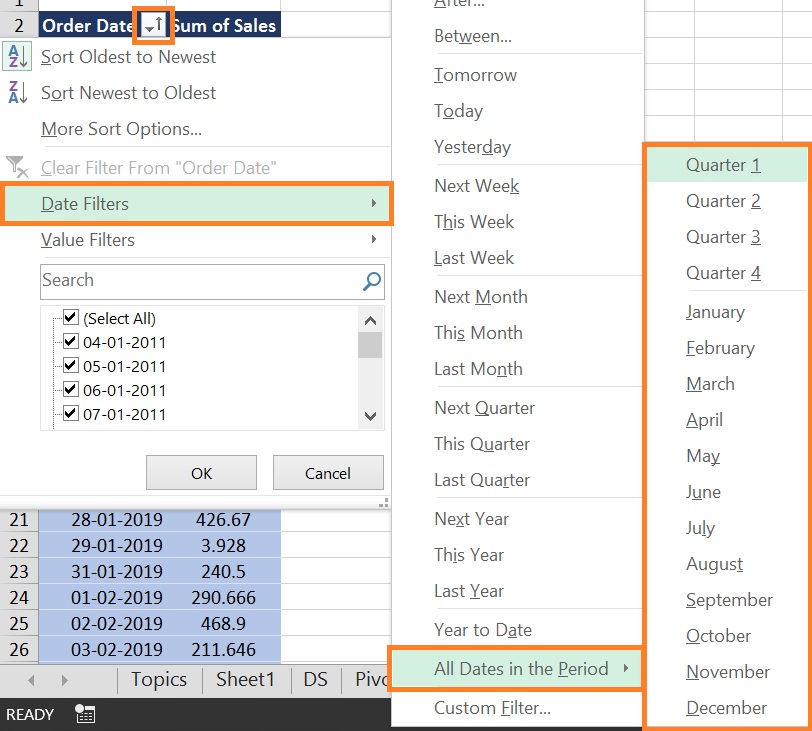
Note: This helps in aggregating data over larger intervals.
The dynamic date range option is not available for pivot fields in the Report Filters area.
Custom Filter
- Where you can define specific criteria for including or excluding dates based on your needs.
- After selecting the desired filter options, The pivot table will update to display data based on the selected date filter.
Using these techniques, you can easily filter data by date within a pivot table to focus on the specific time periods you’re interested in analyzing.
Prevent Date Grouping in Filters
When you create a Pivot Table, Excel groups the dates into months and years. If you want to see individual dates, you will have to change the setting in the Excel option. Follow the below steps to change the setting:
- Go to the file menu then click on “Options”
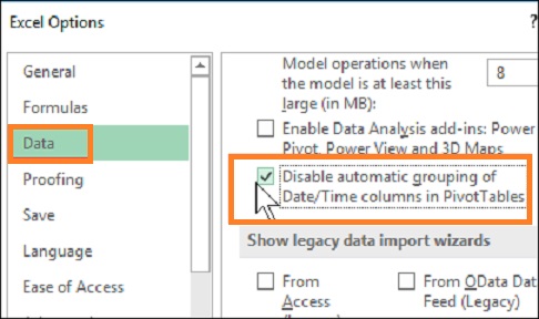
- Click the Data
- In “Data options”, add a check mark to “Disable automatic grouping of Date/Time columns in PivotTables”
- NOTE: If you don’t have that option, you can manually ungroup the dates.
- Click OK to apply the new settings.
NOTE: This is an Excel-Level setting, and will affect all pivot tables that you work on.