HLookup in Excel

How to use HLookup in Excel?

The Letter “H” in HLOOKUP in excel stands for Horizontal Lookup. It is an in-built function in Microsoft Excel that allows you to search a specified value in the first or top row of a table (dataset) and retrieve a value in the same column from a specific row on the bottom side.

When to use HLOOKUP function:

  • If your data is organized in rows with the lookup values in the top row.
  • If you want to find a specific value in that top row and retrieve a corresponding value from a different row in the same column.

The syntax of the HLOOKUP function is:

=HLOOKUP(lookup_value, table_array, row_index_num, [range_lookup])

Here’s what each argument represents:

  • lookup_value: The value you want to lookup/search in the first/top row of the table/range of data.
  • table_array: The table/range of data in which you want to look up the data. The lookup value must always be on the top row in the range of data.
  • col_index_num: The row number in the table/range of data from which to retrieve the matching value.
  • [range_lookup]: This is an optional argument. It is either TRUE or FALSE. The default value is always TRUE means an Approximate match so always use FALSE or 0 for exact matching. For details see the function – VLookup

Example :- Suppose you have sales data of electronics items month wise in which Items are in rows and their monthly sales in columns like below. And I want to quickly track sales of specific products in different months to analyze. 
Then in this case you will have to use the HLOOKUP function to retrieve data. See below snapshot:

HLookup in Excel

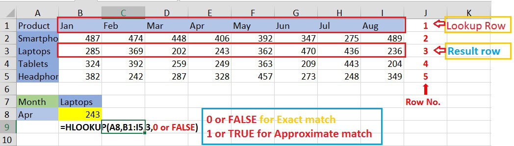
Here HLookup searched “Apr” in 1st row in range “B1:I5” and returned the corresponding value from 3rd row which is 243 using the Exact match option in [range_lookup].

Note: 

  • HLookup can only search for value in the 1st row of table or dataset.
  • If you are searching for approximate match option the data in the first row must be sorted in ascending order but for an exact match the data does not need to be sorted.

HLOOKUP vs. VLOOKUP:

  • HLOOKUP searches horizontally across rows.
  • VLOOKUP, on the other hand, searches vertically down columns.

Tips:

  • Double-check that the data in the top row (header row) of your table is consistent and matches the criteria you’re searching for.
  • Use absolute cell references for the table_array to ensure the formula works when copied to other cells.
  • For approximate matches (using TRUE for range_lookup), ensure your data in the first row is sorted in ascending order.
  • Use error handling techniques like IFERROR or IFNA to manage situations where the lookup value is not found.
  • While HLOOKUP is useful, it has limitations, such as its requirement for the lookup value to be in the first row of the table. Depending on your needs, consider using INDEX MATCH or VLOOKUP if your data is organized vertically and you want to search by a column.

Limitations:

  1. First Row Constraint: HLOOKUP requires the lookup value to be located in the first row of the table array. If the lookup value is in a different row, you’ll need to transpose your data or use a different lookup function.
  2. Exact Match Requirement: For accurate results, you often need to specify an exact match. While this ensures precision, it might not be suitable for situations where approximate matches are acceptable.
  3. Performance: HLOOKUP can be slower than other lookup functions, especially when dealing with large datasets. In such cases, consider optimizing your spreadsheet or using alternative methods.


Hence, The HLOOKUP function in Excel is a valuable tool for performing horizontal lookups, allowing you to retrieve data based on specific criteria from the top row of a table array to streamline your data analysis and decision-making processes.

Related Functions:

Leave a Comment