=VLOOKUP(lookup_value, table_array, col_index_num, [range_lookup])
Here’s what each argument represents:
- lookup_value: The value you want to look up/search in the first/leftmost column of the table/range of data.
- table_array: The table/range of data in which you want to look up the data. The lookup value should always be in the first column in the range of data.
- col_index_num: The column number in the table/range of data from which the matching value should be returned.
- [range_lookup]: This is an optional argument. It is either TRUE or FALSE. The default value is always TRUE means an Approximate match.
- If TRUE ( or “1”) or omitted, an approximate match is returned. If no exact match is found, it will return the closest match which is less than the lookup value.
- If FALSE (or “0”), VLOOKUP will only find exact matches. If there are multiple exact matches, the first found is returned. It’s recommended to use FALSE for exact matching.
Note: In Excel function & formula, the value of TRUE is 1 & the value of FALSE is 0, hence, you can either put the TRUE or FALSE or their value as 1 or 0 instead.
Note: Vlookup doesn’t find the value from the left side of the Lookup Column. Therefore, table_array will be on the right side of the Lookup Column.
In other words, The column in which the lookup value exists must be in the leftmost column of the table or array of data.
(This is the basic concept of VLookup, but we will also find the data from the left side of the Lookup Column with other tactics in this article as well.)
See the example below (table_array is B4:I21) to understand the basics of the VLookup function.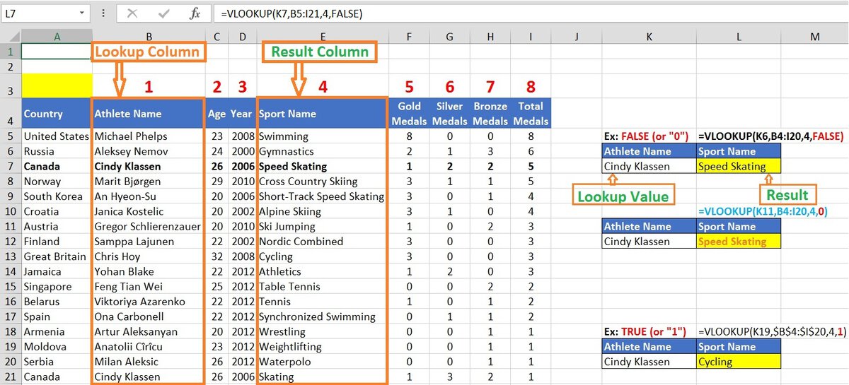
VLOOKUP makes it easy to find exact matches from a table.
To find exact matches using VLOOKUP in Excel, you will need to change the value of [range_lookup] to FALSE (or “0”) because FALSE is used to find the Exact value in the Vlookup function.
Hence, Syntex will be as below:
=VLOOKUP(lookup_value, table_array, col_index_num, [FALSE or 0])
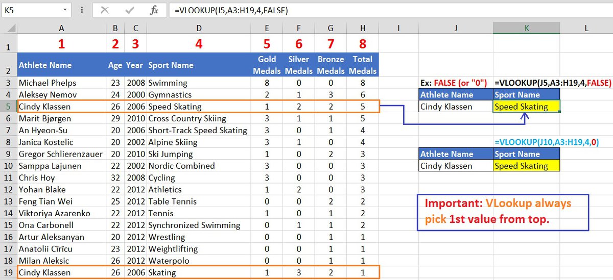
In the example below, the table array is A3:H19 to find spot name with the exact match of Athlete Name “Cindy Klassen” which is in cell J5.
Let’s discuss arguments:
=VLOOKUP(J5,A3:H19,4,FALSE)
- Lookup_value – this argument specifies Lookup Value which is “Cindy Klassen” in cell J5.
- table_array – This argument specifies the table array or Range of data (A3:H19).
- col_index_num – This argument specifies the column index number from where the value should be returned. In the example, the Sport name column is 4.
- [range_lookup] – This Last argument is a Boolean Expression. Here, the value is set to FALSE to return an exact match for the Athlete’s name.
Note: If the exact value is not found then an #N/A error is displayed.
After putting this formula in K5 and pressing enter we get the result as “Speed Skating” which is true.
To find an approximate match using VLOOKUP in Excel, you can follow a similar procedure as with finding an exact match, but you need to set the [range_lookup] argument to TRUE (or “1”) or omit it. Because TRUE is used to find the approximate match value in the VLookup function. It works by finding the next largest value that is less than the lookup value we specify.
Hence, Syntex will be as follows:
=VLOOKUP(lookup_value, table_array, col_index_num, [TRUE or 1 or omit it])
In the example below, this formula will search for the closest match to “Cindy Klassen” in the leftmost column in the table or range of data (A3:H19) and return the corresponding value from the sport name column (column D).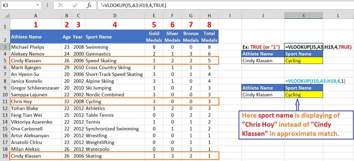
Let’s discuss arguments:
=VLOOKUP(J5,A3:H19,4,TRUE)
- Lookup_value – this argument specifies the Lookup Value which is “Cindy Klassen” in cell J5.
- table_array – This argument specifies the table array or Range of data (A3:H19).
- col_index_num – This argument specifies the column index number from where the value should be returned. In the example, the Sport name column is 4.
- [range_lookup] – This Last argument is a Boolean Expression. Here, the value is set to TRUE to return an approximate match for the Athlete’s name.
After putting this formula in K5 and pressing enter we get the result as “Cycling” which is the sport name of Chris Hoy instead of Cindy Klassen.
VLOOKUP function in Excel is limited to performing lookups based on a single criteria.
If you need to use multiple criteria for a lookup, you will have to create a helping column in which you can combine multiple columns with the help of the concatenate function for the Lookup column.
For example, if you have to look up the Total Medals of Australian players in Swimming, where the country name and sport name are in two different columns, then you will have to use a helping column. This column will store the concatenated values of both columns. See the steps below:
- First, right-click on the Leftmost column header and click on Insert. This will help you insert a column to the left of the Country column.
- for creating the helping column, enter the formula =B3&C3 or =CONCATENATE(B4,C4) in the newly added column and rename this column as you wish. Then, drag the formula down to the rest of the cells in the column.
- On creating the concatenated column successfully, we can now look for the value using this column. Here, we look for the Total Medals of Australian players in Swimming.
- Now Lookup column will be the helping column (Column A)
- So, we enter the formula =VLOOKUP(I7&J7,A3:G19,7,FALSE) in cell K7.
The last parameter is FALSE, as we are looking for an Exact Match. On pressing enter, the Total Medals of Australian players in Swimming will be returned as 3.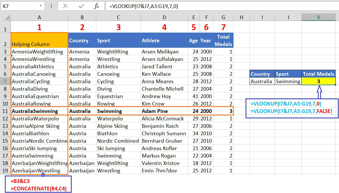
Note:
- You can use this method to Use VLOOKUP for more than two Criteria for a lookup.
- Also, you can use this method when a duplicate value exists in the lookup column to make it unique and find the accurate result.
- Open the worksheet where you want to display the consolidated results. This can be a new sheet or an existing sheet.
- Identify the common field you will use to look up data in the other sheets. This is the field that is common between the sheets. It can be a unique identifier.
- In the worksheet where you want to place the lookup results, enter the VLOOKUP formula in the cell where you want to retrieve the data.
Syntex will be as below:
=IFERROR(VLOOKUP(lookup_value, sheet1!table_array, col_index_num, [FALSE or 0]), VLOOKUP(lookup_value, sheet2!table_array, col_index_num,[FALSE or 0]), …) - Press Enter to enter the formula.
- Once you’ve written the formula in the first cell, you can drag it across other cells in the row or down in the column to apply the formulas to multiple cells.
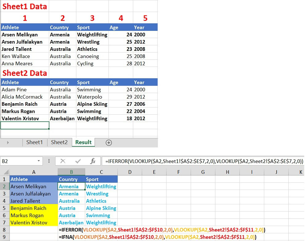
Let’s discuss the arguments:
- Lookup_value – This is the value you want to look up in the table array.
- sheet1!table_array – This is the table array on the first sheet.
- sheet2!table_array – This is the table array on the second sheet.
- col_index_num – This is the column number of the value you want to return.
- [range_lookup] – This Last argument is a Boolean Expression. Here, the value is set to TRUE to return an approximate match.
Tips:
- If you are using the IFERROR function, you can add as many VLOOKUP functions to the formula as needed to look up the value in all of the table arrays.
- You can also use the INDEX and MATCH functions to look up values across multiple sheets. However, these functions are more complex to use than VLOOKUP.
Note:
- Make sure that the common lookup column is in the same position (e.g., column A) in all sheets and that the result column is in the same column index number.
- Make sure that the lookup values in the common column are unique to avoid ambiguity.