What is Pivot Table in Excel?
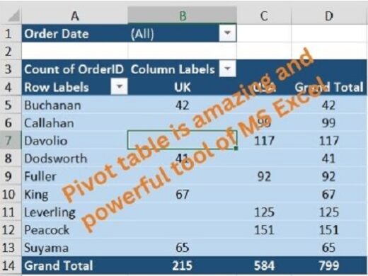
A PivotTable is a strong tool in Excel to summarize and calculate large amounts of data and It can show comparisons and trends in your data. It’s useful if you have a large quantity of data in rows or columns and want to track and compare eye-catching reports painlessly.
Why Pivot Table is used in Excel?
Pivot Table in Excel is used due to below amazing features:
- You can summarize the large data set in a readable form easily.
- You can rotate rows to column or column to row (which is called “pivoting”) to view different summaries or in other words, you can change the structure of the summary table as per needed.
- Pivoting can be done by simply dragging and dropping the column of the source table.
- It can Expand or Collapse the levels of data and drill down to see the details.
- You can filter, group, and sort quickly as per need so that you can focus on the required information.
- It can Subtotal and aggregate numeric data by categories and subcategories as well to analyze.
- There is an option to show blank data as you wish/want in the summary.
Requirements of data set for Pivot Table
The data set for the pivot table must meet the below requirement:
- Organized your data in columns and each column has a single purpose or data item
- Make sure all columns have headers (Also known as Title)
- Headers are always on the top row of data with Unique Level
- Must have non-blank labels for each column means Blank/Empty cells as column header is not allowed.
- Headers must not have merged cells.
How to create/insert/add/make a Pivot Table in Excel?
First of all, select any cell in the data set on which you want to create the Pivot Table then use either the shortcut key or Tool method:
- Using the shortcut: Press ALT then release N, V + Enter
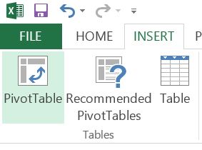
- Using Tool Icon: Go to Insert Menu >> Click on Pivot Table Icon
 from the pivot tables group.
Then you will see the same below dialog box in both methods.
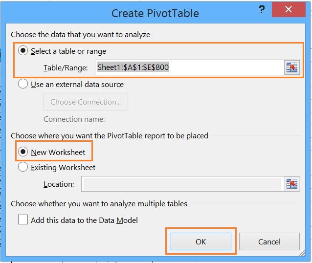
Here you will see the selected data range and if it is not your data range then you can directly resize or reselect your data without going back.
Next, you can select the pivot location where you want to insert the pivot table. in this section you will see 2 options as below:
- New Worksheet >> will create a pivot table in a new worksheet
- Existing Worksheet >> will give you the option to select the location/cells where you want to insert a pivot table in the same worksheet
Next, you can add this data to Data Model by selecting checkbox, if multiple tables are used for pivot.
Then click on the OK button and you will see Blank Pivot Table with Pivot Table Fields option as below
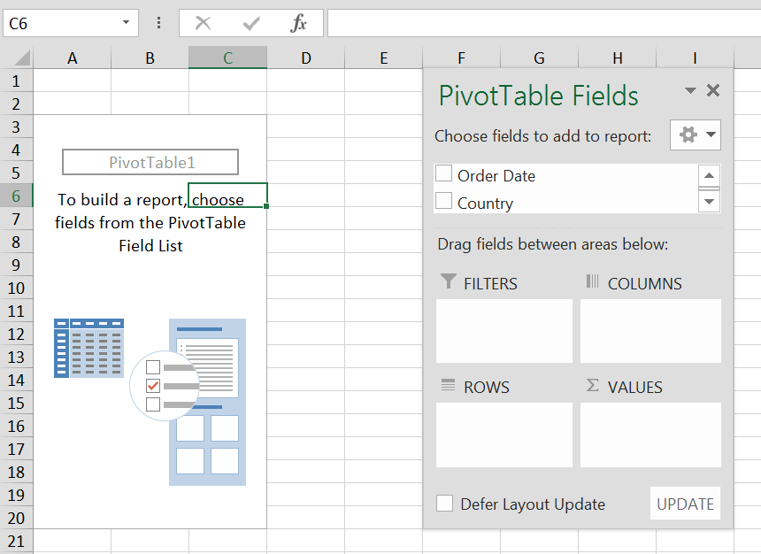
Now you will have to drag the fields from choose fields to add to the report section in the below section where you will get 4 options.
Let’s discuss these options:
Pivot Table Fields elements
- FILTERS – Put the field here to apply any filter on data that will show above the pivot table.
- COLUMNS – Put the field here that you want to keep in the column on top of the pivot table report
- ROWS – Put the field here that you want to show row-wise on the left side of the pivot table in the report
- VALUES – put the field here to get summarized numeric values like count, sum, average, percentage, etc. in the report.
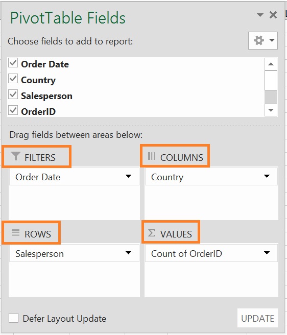
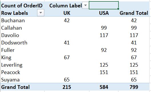
Note: If you want to add more than one field in any area or section you will have to re-arrange the order of fields by dragging the field in that particular section. finally, you will get the below summary:
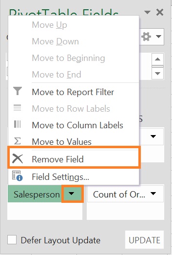
How to remove fields from the Pivot Table?
If you want to delete/remove fields from the pivot table then drag that field out of its area. Also can be removed by clicking the down arrow next to the field, then selecting Remove Field.
Why is Pivot Table called Pivot?
Usually, the user rotates the field or changes the structure of the summary in the pivot table by dragging and dropping fields graphically from row to column or column to row, that concept is called “pivoting” or “Pivot“.
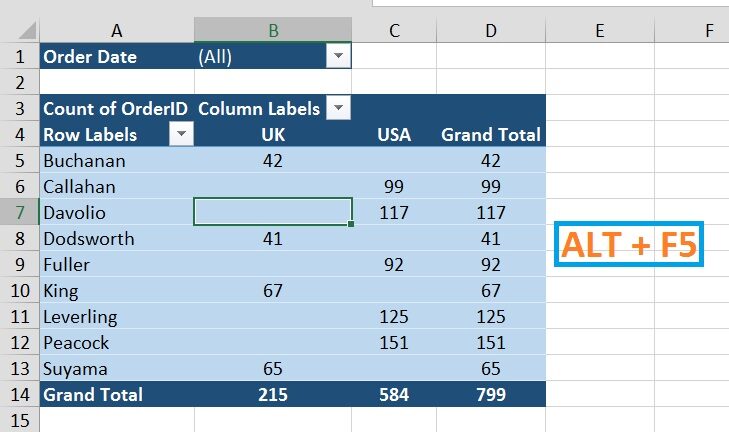
How to Refresh the Pivot Table in Excel when source data changes?
There are many methods to refresh the pivot table to get the latest data from the source dataset
- Click anywhere on the Pivot Table then Press ALT+F5
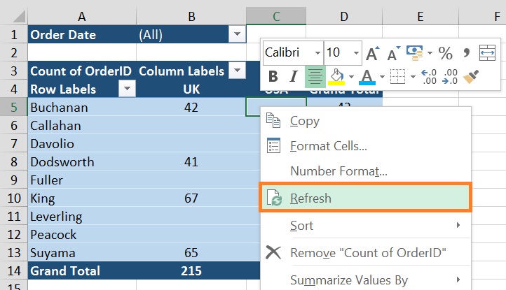
- Right-click on the pivot table then select Refresh.
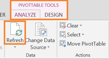
- Click anywhere on the Pivot Table then you will see the PivotTable Tools menu on the ribbon
> Click on ANALYZE TABLE
> Then click on the Refresh icon directly available under the “Data” group
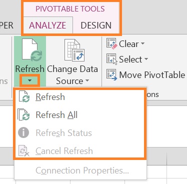
Also, you will get some Refresh Options if you click on the dropdown of the Refresh icon:
- Refresh (Alt+F5) >> It will refresh the pivot table that is in the active cell. This means you will get the latest data from the source.
- Refresh All (Ctrl+Alt+F5) >> It will refresh all the pivot tables and you will get the latest data from all sources. It takes refreshing time longer than you expect.
- Refresh Status >> If refreshing takes longer than you expect then you can check the status by clicking Refresh Status
- Cancel Status >> It is used to stop Refreshing the pivot.
To know about Refresh data Automatically when opening the workbook, click here.
How to Delete or Remove Pivot Table in Excel?
If you want to delete or remove the pivot table from Excel, you will have to follow one of the steps below:
1. Select the Entire Pivot Table then press the Delete key from the keyboard.
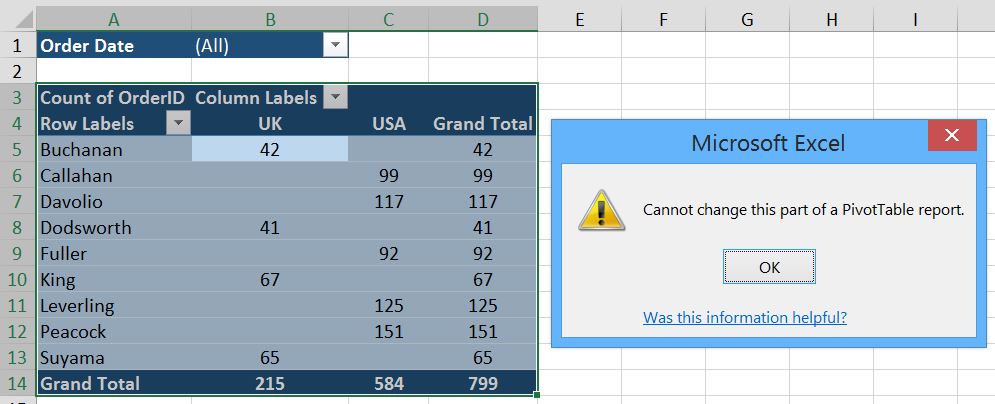
Note: If you get a message like “Cannot change this part of a PivotTable report.”, then make sure the entire PivotTable is selected.
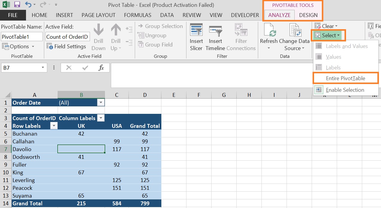
2. Click anywhere on the Pivot table to show the PIVOT TABLE Tools menu on the ribbon
> Click on analyze tab > Go to action group > Click on Entire PivotTable
> Press the Delete key from the keyboard
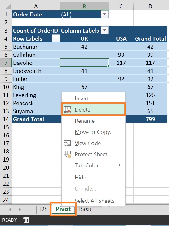
3. If PivotTable is on a separate sheet where no other data you want to keep then delete that sheet. this is a fast-forward way to remove the Pivot Table.
Note: You can delete the sheet in many ways. (1.) Using the mouse – Right-click on the sheet tab then select the Delete option. (2.) Using Shortcut – Press ALT then release, then H, D, S.
Hope this post will be helpful if exploring about Pivot table.