Filter data in Pivot Table
Filter data in Pivot Table in Excel is used to quickly focus on specific data in your pivot table summary. It can be filtered by date, value, top or bottom rankings, and many more.
Contents
ToggleTypes of Filters in a Pivot Table
There are many options to filter data in the pivot table in Excel. See the below for all the levels of filters and try to understand the uses of these options.
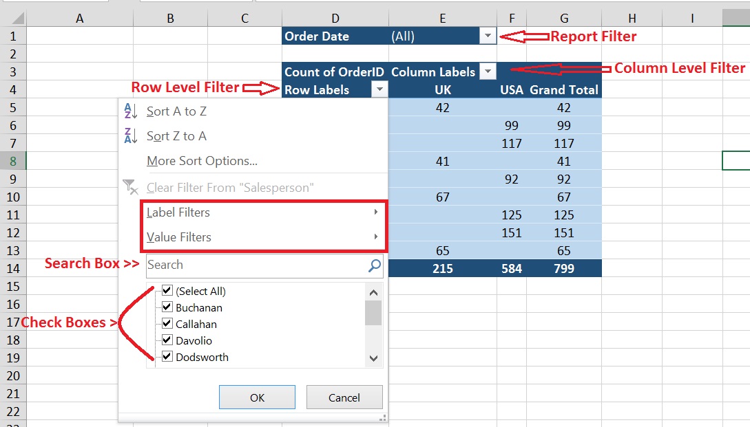
- Report Filter
- Row/Column Labels Filter – Following types of filters are available in it:
- Label Filters – used to filter by string/Text
- Value Filters – used to filter value/number
- Date Filters – used to filter date when date data in row/column
- Common Filters in Report Filters & Row/Column Labels
- Filters using Search Box – whatever data in column
- Filters using Check Boxes – by checking or unchecking box
Report Filter
By utilizing a report filter, you can rapidly show an alternate arrangement of values in the PivotTable. Things you select in the filter are shown in the PivotTable, and things that are not selected will be hidden. You can create this filter by dragging and dropping the field into the Filters area in the pivot table.
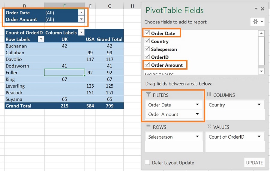
Add a report filter
- Click anywhere in the pivot table
- Pivot Table Fields Pane will appear
- click on the field in the area “Choose fields to add to report” and move to the filters area by drag and drop.
Note: In the Filter area, you can change the order of the fields by either dragging the fields to the desired position or clicking on a field in the Filter area and selecting Move Up or Move Down. The order of the report filters will be reflected accordingly in the Pivot Table.
Display report filters in rows or columns
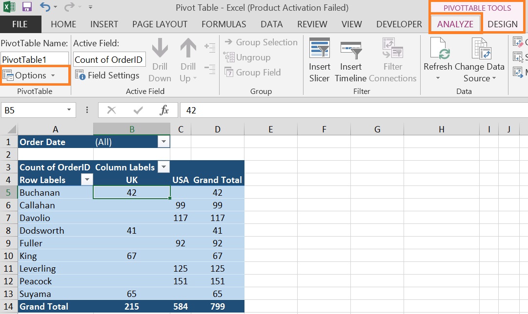
- Click anywhere in the pivot table
- Click on ANALYZE tab under PivotTable Tools
- Click on Option in PivotTable Group
- PivotTable Options dialog box will appear
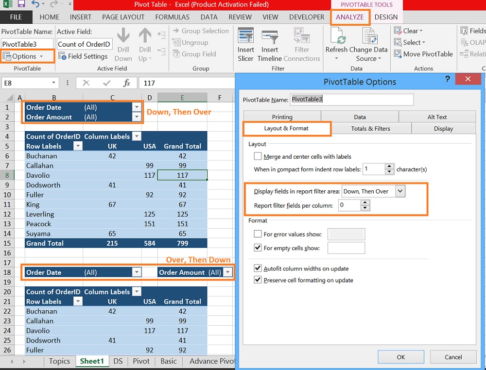
- click on Layout & Format tab
- Select one of the following from drop down in Display fields in report filter area:
a. Down, Then Over: to display report filters in rows from top to bottom
b. Over, Then Down: to display report filters in columns from left to right - Report filter fields per column: 1,2,3, ….
- Select one of the following from drop down in Display fields in report filter area:
Select items in the report filter (Search & Check Box)
- Click on the dropdown arrow next to the report filter
- A new dialog box will appear to select items
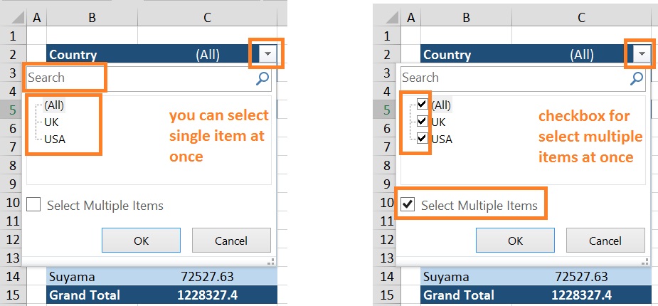
- Tick on Check Box of any one item to appear with details of that item in the Pivot Table or by searching item from the Search box
- Select Multiple items – Tick on the checkbox, It will provide the facility to select multiple items at once.
- tick all those items, you want to display in the report or select All to display all items in Pivot Table.
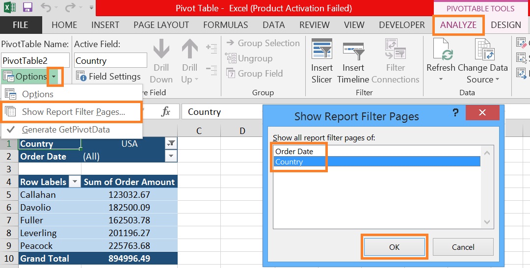
Display report filter pages on separate worksheets
- Click anywhere in the pivot table
- Click on ANALYZE tab under PivotTable Tools
- Click on dropdown next to Option in PivotTable Group and then
- select “Show Report Filter Pages…”
- A New dialog box appear, select a report filter field, and then click OK.
- now you will get the same filtered report in new worksheet.
- so select one by one and follow same steps for others items in filter if required.
Column or Row Labels Filter
These filters allow you to filter specific data in the pivot table based on the field items.
Like a specific item or item that contains a specific text or the values like top 10 items by value or items with a value greater than or less than a specified value.
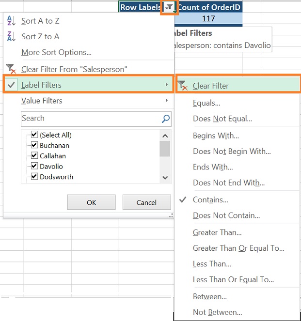
Label Filters
- Select the Filter drop-down arrow next to row/column labels, which varies depending on the report layout.
- To filter by creating a conditional expression, select Label Filters, and then create a label filter.
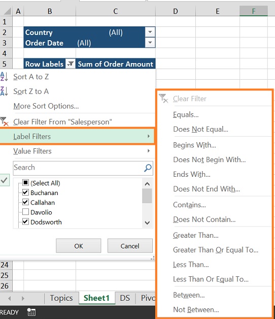
Value Filters
- To filter by values, select Values Filters and then create a values filter.

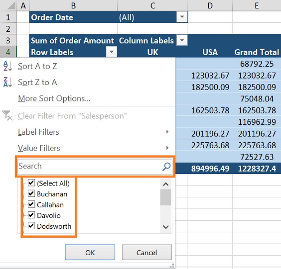
Search Box & Check Boxes Filters
Search Box: You can access Pivot Table filters within the row/column label filter and this allows you to quickly filter based on the text you enter. For example, if you want to show data for Callahan only, just type Callahn and it will filter that for you.
Check Boxes: These allow you to select specific or multiple items from a list. For example, if you want to analyze for Callahan only, you can do this here. Alternatively, you can also include some more items by checking the tick box or exclude some items by unchecking it.
- To filter by specific row labels or column labels, first, uncheck (Select All), and then select the check boxes next to the items you want to show. You can also filter by entering text in the Search box.
- Click OK.
Clear Filter from a Row or column Labels
Method - 1
- Click on the arrow next to the row/column Label.
- Click on Clear Filter From “<Field Name>” to change or clear the filter.
Note: If one or more items are selected then it will show for Clear Filter and if checked (Select All) then It will gray out and will not work.
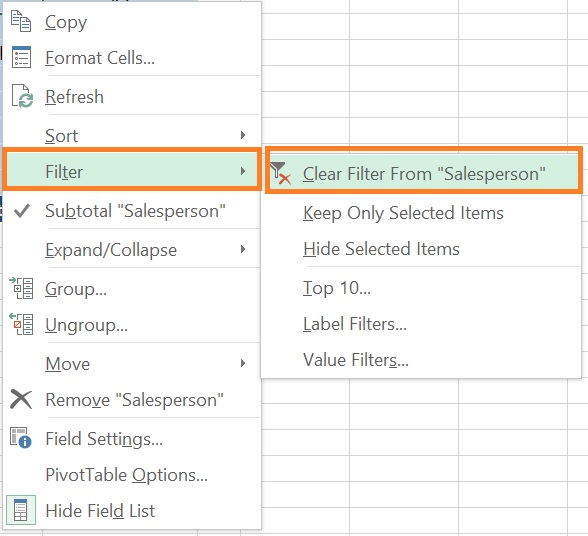
Method - 2
- Right-click on the row/column where you have applied the filter
- then select “Filter”
- Then click on Clear Filter From “<Field Name>”.
Method - 3
- Click on the arrow next to the row/column Label
- Then click Label Filters/Value Filters/Date Filters, whatever filter is applied in your case
- Then click on Clear Filter.
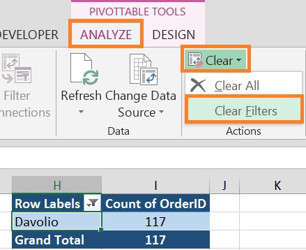
Method - 4
If you want to clear all the filters of the Pivot Table irrespective of columns and rows, follow the below steps:
- Click on the pivot table to activate the Analyze tab in PivotTable Toos menu
- Now, click on the little down arrow next to Clear in the Actions group tool
- Then click on “Clear Filters”. This will clear all the filters applied to the pivot table (in other words, it will reset the filters).
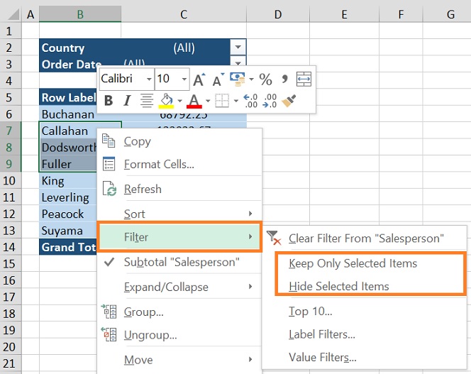
Filter by selection to display or hide selected items only
- Select one or more items in the field in pivot table filter that you want to filter by selection
- right-click an item in the selection
- Click on Filter
- Then select one of the following:
- Keep Only Selected Items – It will show the selected item(s) and rest will hide.
- Hide Selected Items – It will hide the selected item(s)
Turn Filtering options On or Off
If you don’t want to show the filter dropdown arrow to prevent filtering in your pivot table then you can do it by following the below steps
- click anywhere in the pivot table then it will show PivotTable Tools tab on the ribbon.
- go to analyze tab
- click on Option in PivotTable group
- now PivotTable option dialog box will appear
- Click on the display tab
- unselect “Display field caption and filter drop downs” to hide field captions and filter drop downs.
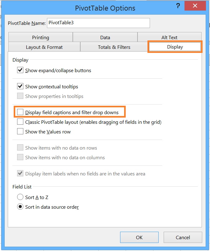
- If you want to show Filter dropdown arrow to Filter Data then select “Display field caption and filter drop downs”.