Slicer in Excel

What is a Slicer in Excel?

A slicer in excel is a user interface (UI) feature used primarily on Tables, Pivot Tables, and Pivot Charts to filter data and perform interactive analysis on large amounts of data. It provides buttons that you can click on to filter the data.

In addition to quick filtering, slicers also indicate the current filtering state, making it easy to understand what exactly is currently being displayed.

These are commonly used for data visualization and dashboard creation that display tabular summary reports. You can connect multiple slicers to multiple pivot tables to create reports.

But remember that slicers are mainly for user interaction and filtering data in PivotTables and PivotCharts. They don’t change the underlying data; instead, they help you view subsets of data more easily.

How to use Slicer in Excel?

Adding slicers to Excel is a straightforward process, and it can greatly enhance the interactivity of your Table, Pivot Tables, and Pivot Charts. Here’s how to use or add a slicer in Excel:

Three steps can be followed to insert a slicer in an Excel Table, Pivot Table, or Pivot Chart and use it.

  1. Convert your data to tabular format (Table), Pivot Table, or Pivot Chart format.
  2. Select any cell of the Excel Table or pivot table and insert the slicer.
  3. Use the Slicer.

Step - 1: Create a Table, Pivot Table or Pivot Chart

By default, Excel treats your data as a database, and adding slicers will not be possible. So in order to insert or create a slicer, you will need to convert your data into a simple Excel Table or Pivot Table or Pivot Chart.

To Create a Excel Table

To create a simple Excel Table follow the steps below:​

  • Select the range of data you want to analyze.
  • Press Ctrl+T keys to convert your data into a table
    or
    Click on the Table” icon from the Insert” menu.
  • Select the table range and click “OK”.

For details go through with article Benefits to use Excel Table.

create a Table for Slicer

To Create a Pivot Table

To create a Pivot Table follow the steps below:​

  • Select the range of data you want to analyze.
  • Press Alt, N, V or in the latest version press Alt, N, V, T keys to convert your data into a Pivot Table
    or
    Click on the
    Pivot Table” icon from the “Insert” menu.
  • In the PivotTable dialog box, make sure the data range is selected correctly and choose where you want the PivotTable to be placed (e.g., a new worksheet or an existing one)
  • Select the table range and click “OK”.

For details go through with article Pivot Table in Excel – Easy to understand.

To Create a Pivot Chart

To create a Pivot Chart follow the steps below: (Also you can create a Pivot Table by these steps)

  • Select the range of data you want to analyze.
  • Go to the “Insert” tab in the Excel ribbon
  • Go to the Charts group.
  • Select “PivotChart” or “PivotChart and PivotTable” from drop-down on “PivotChart”.
  • In the PivotTable or PivotChart dialog box, make sure the data range is selected correctly and choose where you want the PivotTable or PivotChart to be placed (e.g., a new worksheet or an existing one)
create a Pivot Chart for Slicer
  • Click “OK” to create the PivotTable or PivotChart.
Chart on Pivot Table

Step - 2: Add Slicers

Once you have your Excel Table, PivotTable or PivotChart in place, you can add slicers to filter data quickly:

Create Slicer on Excel Table

Create a slicer to filter data in an Excel Table, follow the steps below:

      • Select any cell of the Excel Table
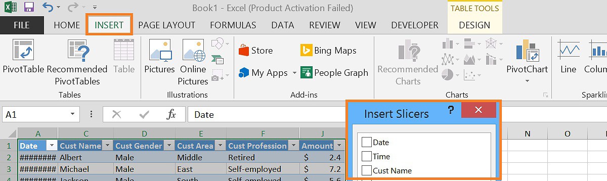
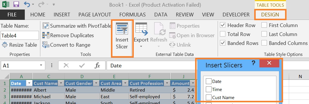
      • Go to “Insert” Menu and click on Slicer from the “Filters” group

        Create a slicer on Excel Table from Insert menuOR

      • The “Design” menu under “TableTools” will activate, then click Insert Slicer from the “Tools” groupCreate a slicer on Excel Table from Design menu.

Create Slicer on Pivot Table or Pivot Chat

Create a slicer on Pivot Table or Pivot Chat, follow the steps below:

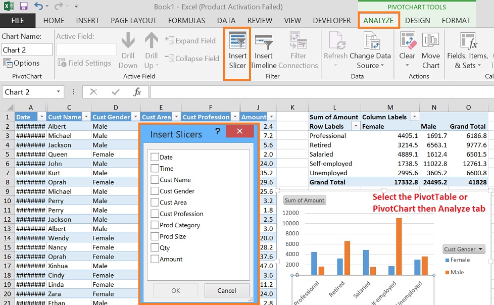
  • Select the PivotTable or PivotChart if you want to add slicers. You’ll notice that the “PivotTable Analyze” or “Chart Design” tab appears in the Excel ribbon when you have a PivotTable or PivotChart selected.
  • Go to Insert Menu in the ribbon and click on Slicer from the Filters group.
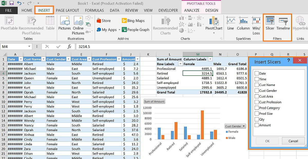
    Create a slicer on Pivot Table or Pivot Chat from Insert menu
    OR

  • Click on the “Insert Slicer” button in the “Filter” group on the “PivotTable Analyze” or “Chart Design” tab. This will open the “Insert Slicers” dialog box.

    Create a slicer on Pivot Table or Pivot Chat from Analyze
    .

Insert Slicers dialog box

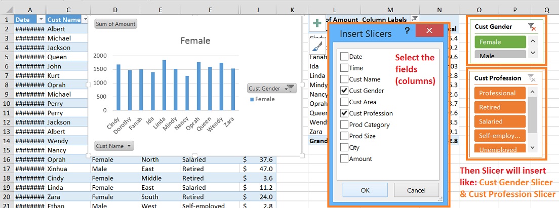
  • In the “Insert Slicers” dialog box, select the fields (columns) from your data that you want to use as slicers. You can select multiple fields if needed.
  • Click “OK” to insert the slicers into your worksheet like in below image (Cust Gender & Cust Profession).

    Slicers in excel

Step - 3: Use the Slicers

Once you add slicers, they will appear as interactive filter controls in your worksheet. To use them:

  1. Click the slicer button to select or deselect items. This will instantly filter the data in your PivotTable or update your PivotChart to show only the selected items.
  2. To select multiple items in a slicer, hold down the Ctrl key (Command key on Mac) while clicking the items you want to include in the filter.
  3. To clear a slicer’s filters and show all data again, click the “Clear Filter” button (usually represented as a red “x” or “clear” icon) at the top of the slicer.
  4. You can use multiple slicers together to create more complex filters, and the data will update dynamically as you select.
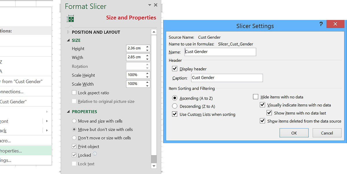
  5. Customize the slicer appearance and layout by right-clicking the slicer and selecting “Slicer Settings” or “Size and Properties” depending on your version of Excel.
    Slicer Settings dialog box

That’s it! You’ve added slicers to your Excel worksheet, and now you can use them to easily filter and interact with your PivotTable or PivotChart data.

The benefit of using a slicer in Excel

The Slicer is a powerful feature in Microsoft Excel that provides many benefits when working with PivotTables and PivotCharts. Here are some of the key benefits of using the slicer in Excel:

  1. User-Friendly Filtering: Slicers provide a user-friendly way to filter data in Pivot Tables and PivotCharts. Instead of navigating through complex filter menus, users can simply click the slicer button to filter data quickly and intuitively.
  2. Visual Representation: Slicers provide a visual representation of the available filter options. Users can see at a glance which items are selected and which are not, making it easier to understand the current data subset.
  3. Interactivity: Slicers add interactivity to Excel reports. Users can easily switch between different filter selections, allowing dynamic exploration of data without the need to manually adjust filter criteria.
  4. Multiple Selections: Slicers allow multiple selections, making it convenient to filter more than one item at a time. This is especially useful when analyzing complex datasets with many categories or values.
  5. Customization: Excel provides options to customize the appearance of the slicer, including changing the style, size, and layout. You can match the slicer to the overall design of your report or dashboard.
  6. Connected Slicers: You can create multiple slicers that are connected to each other. This means that selecting an item in one slicer can automatically filter the available options in the other slicer, which can be very useful for digging deeper into the data.
  7. Compatibility with PivotCharts: Slicer can be used with PivotCharts to create interactive dashboards. When you select an item in the slicer, the associated PivotChart will update to reflect the filtered data.
  8. Clear Reset Options: Slicers often include a “Clear Filter” button  (a red x) at the top of the slicer, allowing users to easily reset the filters and view the entire dataset again. This is especially useful when users want to start a new analysis.
  9. Print and Export: Slicers also work well when printing or exporting Excel reports. They provide a clear way of showing which filters have been applied, helping to maintain transparency in your data presentations.
  10. Accessibility: Slicers are accessible to users with disabilities and are compatible with screen readers, ensuring everyone can interact with your data effectively.
  11. Time Efficiency: Slicers can save time for both data analysts and end users. Analysts can create slicers once, and users can filter data without in-depth knowledge of Excel’s filtering options.

In summary, Slicers in Excel is a user-friendly and visually attractive way to filter and interact with data in PivotTables and PivotCharts. They enhance the usefulness and interactivity of Excel reports and dashboards, making it easier for users to analyze and explore data effectively.

Slicer Components

A slicer displays the components as below:

Slicer Components

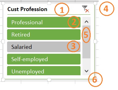
  1. Header – A slicer header indicates the category of the items in the slicer.
  2. Button selected – A filtering button that is selected indicates that the item is included in the filter.
  3. Button unselected – A filtering button that is not selected indicates that the item is not included in the filter.
  4. Clear Filter – A Clear Filter button removes the filter by selecting all items in the slicer.
  5. Scroll Bar – A scroll bar enables scrolling when there are more items than are currently visible in the slicer.
  6. Border – Border moving and resizing controls allow you to change the size and location of the slicer.

Customize or Format the Slicer

The formatting options for slicers can enhance their appearance and usability in your Excel workbooks.

Slicer Styles

Change the Slicer Styles

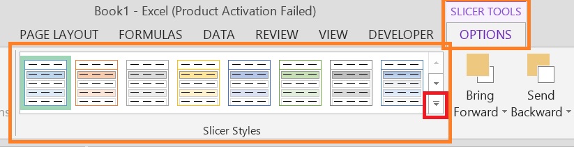
  • On the “Slicer Tools” contextual tab, go to the “Options”.
  • Use the “Slicer Styles” dropdown to apply a pre-defined style to your slicer. These styles include various color schemes and designs.

Slicer Styles in excel

Customize Slicer Styles (i.e. Font, Border Color, Background Color, etc.)

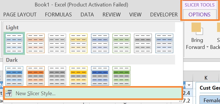
If you want to further customize the appearance of the slicer,

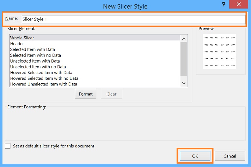
  • click the “Slicer Styles” dropdown, then select “New Slicer Style”.

New Slicer Style option

  • Click on ”Format” in the “New Slicer Style” dialog box, and you can modify various formatting options, such as the slicer’s font, border, border color, background color/effect/pattern, and so on from “Format Slicer Element” dialog box.

Format Slicer Element dialog box

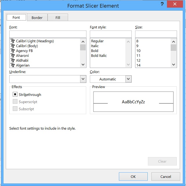
  • To change a specific color element, select it from the list on the left side of the dialog box and choose a new color using the color picker.
  • Preview your changes as how the slicer will look by viewing the changes in the preview area on the right side of the dialog box.
  • You can also set a specific modified style as the default slicer style for this document by checking the “Set as default slicer style for this document” box.

New Slicer Style Dialog box

Save or Name your Custom Slicer Style

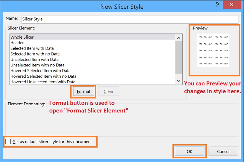
  • Give your custom slicer style name in the “Name” box, available on top of new slicer style dialog box.
  • Click the “OK” button to save your custom style.

Name your Custom Slicer Style

Apply the Custom Slicer Style

  • After creating your custom slicer style, it will be added to the list of slicer styles so you can apply it to your slicer by selecting it from the “Slicer Styles” dropdown on the “Slicer Tools” tab.

Size and Properties of Slicer

Getting Multiple Columns in the Slicer Box

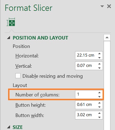
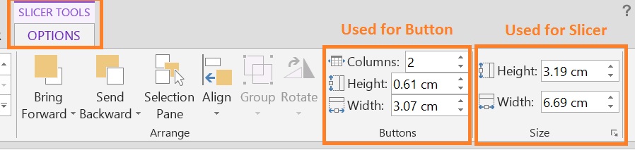
By default, a Slicer has one column, and all items of the selected field/column are listed in it. In case you have many items, Slicer shows a scroll bar that you can use to move to all the items.

You may want to have all the items visible without the hassle of scrolling. You can do this by creating multiple columns Slicer.

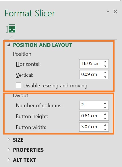
  • By changing the Number of columns under the Position and Layout section accessed from size and properties by right-clicking.
    Getting Multiple Columns through right click from position and layout
    Or
  • Optionally, Select the Slicer then Go to “Slicer Tools” and choose Options.
  • In the “Buttons” group, change the Columns value to 2 or whatever you want.
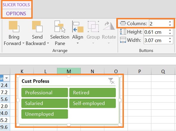
    Getting Multiple Columns in the Slicer Box
    .
  • This will instantly split the items in the Slicer into two or the desired number of columns.

This looks disorganized and full names are not displayed. To make it look better, you can change the size of the slicer and even the buttons of it.

Height & width of the Buttons and the Slicers

  • Select the Slicer then go to “Slicer Tools” and choose Options.
  • Change the Height and Width of the Buttons and the Slicers. (Note: You can also change the size of the slicer by simply selecting it and using the mouse to adjust the edges. However, to change the size of the button, you just have to change from the Options only).
  • The height and width of the slicer can be changed by the size and properties of the slicer.
    Height & width of the Buttons and the Slicers


Resize and Position the Slicer

  • Click and drag the border of the slicer to resize it.
  • Click and drag the slicer to reposition it within the worksheet.    or
  • Optionally, From the Position and Layout section in Size and Properties.
    Resize and Position the Slicer


Lock or Hide Slicer Elements

  • To prevent users from modifying slicer selections, you can lock the slicer.
  • Right-click on the slicer and select “Size and Properties”.
  • In the “Properties” window, add check mark in the “Locked” box.
    Lock or Hide Slicer Elements

How to unlock the Slicer in a protected worksheet

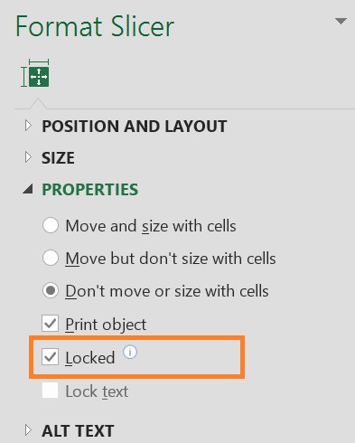
When sharing your worksheet with other users, you might want to lock your pivot tables from editing, but keep the slicer selectable.

  • To unlock more than one slicer at a time, hold down the Ctrl key while selecting a slicer.
  • Right-click on any selected slicer and select “Size and Properties”.
  • On the Format Slicer pane, under Properties, uncheck the Locked box, and close the pane.
  • On the Review tab, in the Protect group, click Protect Sheet.
  • In the Protect Sheet dialog box, check the Use PivotTable & PivotChart option.
    ProtectSheet dialog box for slicer
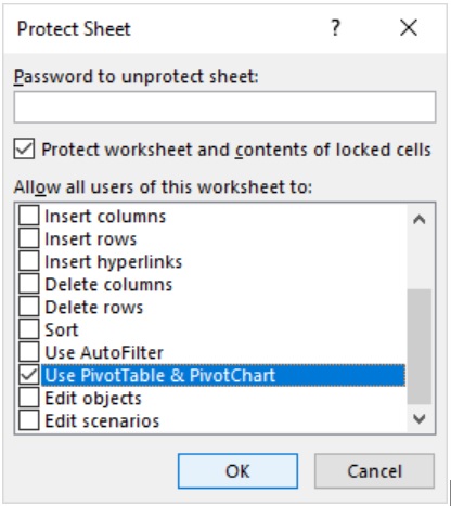
  • Enter a password or leave it blank and click OK.

Change the slicer settings

Removing the Slicer Header

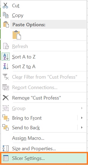
  • Right-click on the Slicer then select Slicer Settings.
  • Remove the check from the Display Header option in the dialog box.
    Removing the Slicer Header


Change the Slicer Caption or Header Name

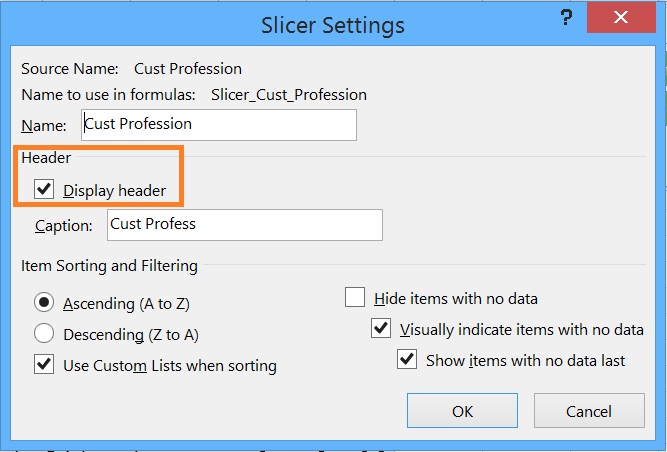
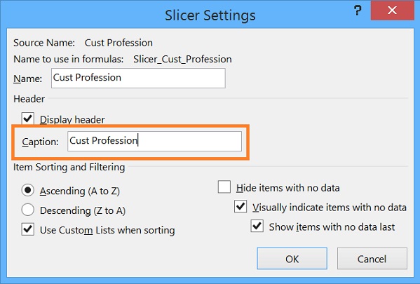
By default, a Slicer selects the field name from the source data. You may want to change the header,

  • You can edit the slicer’s caption by selecting the slicer then clicking on the caption text, and then typing in the new caption.
    Caption or Header Name of slicer
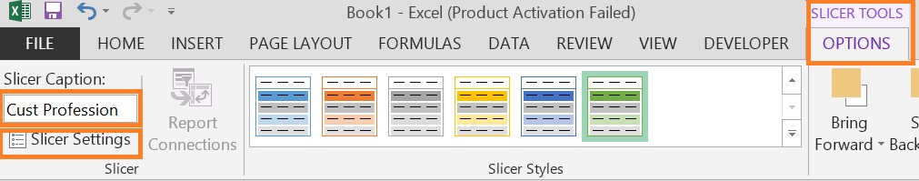
  • Select Slicer Settings from the Slicer Option in the Slicer group or Right-click over the Slicer.
    Caption or Header setting by right click
  • In the Slicer Settings dialog box, change the header caption to whatever you want. This will change the header name in the slicer.
    Slicer setting for Caption or Header Name

Sorting Items in the Slicer

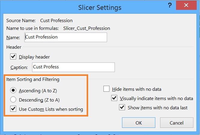
By default, the items in the slicer are sorted in ascending order in the case of text and Older to Newer in the case of numbers/dates.
You can change the default settings and even use your own custom sort criteria.

  • Right-click on the Slicer and select Slicer Settings.
  • In the Slicer Settings dialog box, you can change the sorting criteria, or use your own custom sorting criteria.Sorting Items in the Slicer

Hide Items with No Data from the Slicer Box

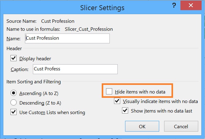
It may happen that some items in the pivot table do not contain any data. In such cases, you can hide that object from the slicer.

  • Right-click on the Slicer that contains the data you want to hide then select Slicer Settings.
  • In the Slicer Settings dialog box, with the “Item Sorting and Filtering” options, check the “Hide items with no data” option.
    Hide Items with No Data from the Slicer Box

Connect Slicer to multiple pivot tables and charts

If you already have a slicer on a pivot table, you can use the same slicer to filter another pivot table.

Note: Slicers can only be connected to PivotTables that share the same data source.

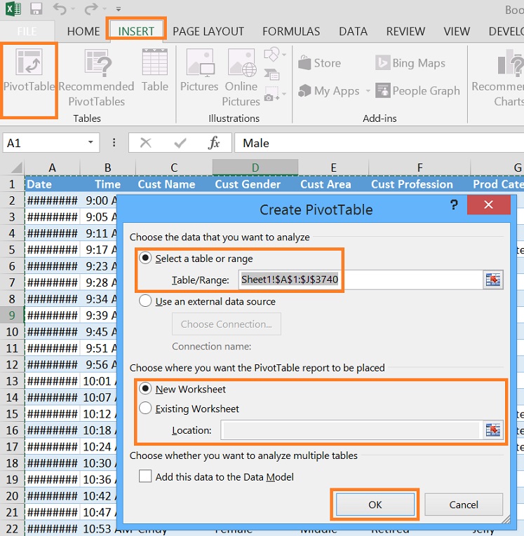
  1. First, create a Pivot Table based on the same data source as the PivotTable that already has the slicer you want to reuse
    or Create two or more pivot tables, ideally, in the same sheet.
  2. Give your pivot tables meaningful names so that you can easily identify each table by its name. To name the pivot table, go to the Analysis tab and type a name in the PivotTable name box in the upper left corner.

    Note: If you don’t give meaningful names to your pivot tables, Excel will give them default names like PivotTable12. It can be confusing once you have more pivot tables.

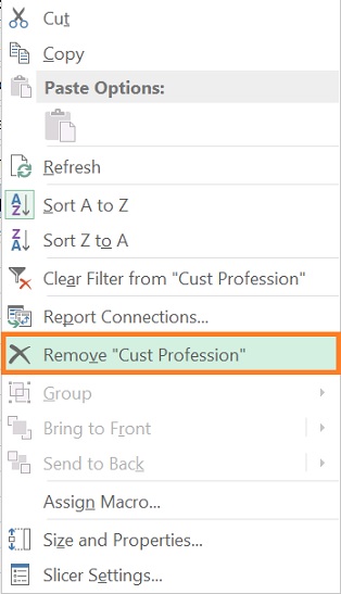
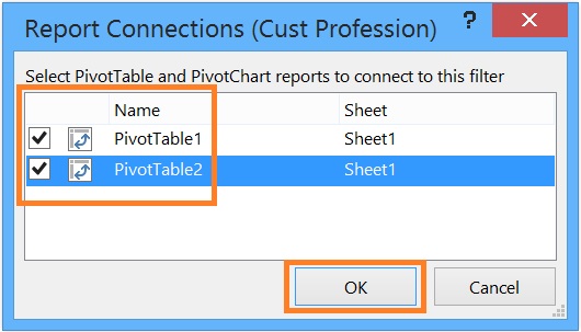
  3. Right-click on the slicer, and then click Report Connections
    Report Connections Through Right Click
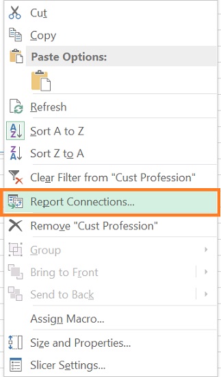
    Alternatively, select the slicer you want to share with another pivot table. This displays the Options under the Slicer Tools tab.
  4. On the Slicer group, select Report Connections.
    Report Connections in slicer
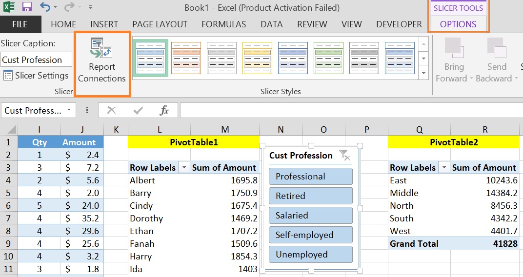
  5. In the dialog box, select the check box of the Pivot Table in which you want the slicer to be available. Now both pivot tables will respond to the slicer.
    Report Connections Dialog box in excel
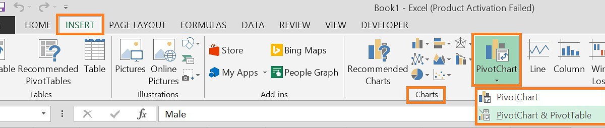
  6. You can use the same approach to link a slicer to more than one chart (pivot chart or regular chart).

Disconnect a slicer

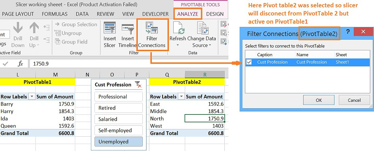
  1. Click anywhere in the Pivot Table from which slicer you want to disconnect. This displays the Pivot Table Analysis tab.
  2. Select the Pivot Table Analyze tab, and then select Filter Connections from the Filter group.
  3. In the dialog box, clear the check box of any Pivot Table fields for which slicer you want to disconnect the slicer.
    Disconnect a slicer

Delete a slicer

  • Select the slicer, and then press Delete.
  • Right-click on the slicer, and then select Remove “Name of Slicer”.
    Delete a slicer

Excel Slicers vs. Pivot Table Filters or Report Filters

There are some key differences between both as below:

  • Pivot Table Filters are tied to the single pivot table. Slicers can be linked to multiple pivot tables and pivot charts.
  • Pivot Table Filters are difficult to work with as there are too many options in terms of labels and value filters. You need to choose criteria based on how the filtered table will appear. With Slicer, filtering pivot tables is as easy as just clicking a button.
  • Filters are locked on columns and rows. Slicers are floating objects and can be moved anywhere.
  • Pivot Report Filters may not work very well in a touch screen environment. Slicers perform well in many touch-screen environments, except Excel Mobile (including Android and iOS), where this feature is not fully supported.
  • Report filters take up one cell per filter. Slicers take up more space on the worksheet.
  • Pivot table filters can be easily automated with VBA. Automating the slicers requires a little more code.

FAQs

Yes, you can insert a slicer without a pivot table, although you must have an Excel table to insert the slicer.

You can use the Slicer Multi Select button to filter by multiple criteria at the same time. 
Once you’ve set up your slicers, simply click the Multi-Select button. (It’s the button with three check marks at the top of the dashboard) You will then be able to filter by multiple criteria.

Yes, you can. Right-click on the slicer and go to “Slicer Settings”. Uncheck the “Display Header” option to remove the header & clear the filter button.
For details see the above section – Removing the Slicer Header.

Right-click on the slicer and choose “Slicer settings”. Check the “Hide items with no data” option. For details see the above section – “Hide Items with No Data from the Slicer Box”

Leave a Comment