Value Filter in Pivot Table in Excel

Value Filter in Pivot Table

Value filter in Pivot Table is a tool used to filter and display specific data based on the values in one or more columns or fields within the pivot table. This filter allows you to focus on specific data points or ranges that meet certain criteria, helping you analyze your data more effectively.

1. Filter Top 10 Items in Pivot Table

You can use Top 10 filter in a pivot table to filter

  • Top or Bottom items by value
  • Filter Top or Bottom Items that make up a Specified Percent of the Value
  • Filter Top or Bottom Items that make up a Specified Value (Sum)

Top or Bottom items by value

Filtering the top or bottom items by value in a pivot table allows you to focus on the most significant or least significant data points in your dataset.

1. Filter a Pivot Table for Top 10 Items
  1. You can use Top 10… Filter feature in a pivot table to focus on specific portion (i.e top/bottom 10 or 2,3,4,5….(n)) of top or bottom items or items that make up the specific percent. 
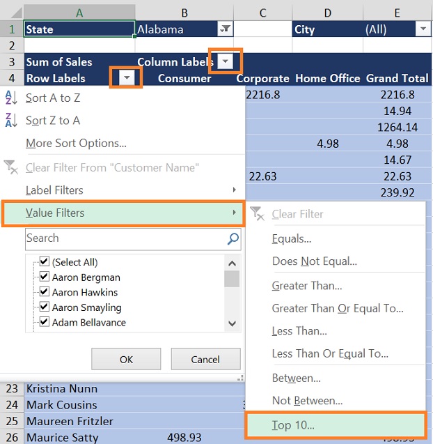
    Use the following steps:
  2. Click the drop down arrow next to Row Level or Column Levels.
  3. In the pop-up menu, click Value Filters
  4. then click Top 10…

Top 10 Filter in pivot table in excel

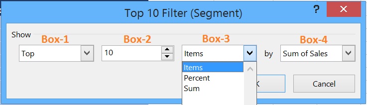
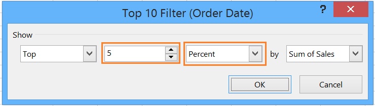
A New Top 10 Filter Dialog box will appear with four columnsSee details below for these all columns or boxes:
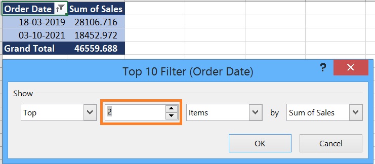
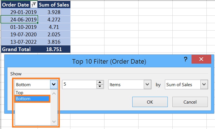
  1. In the first box, select Top or Bottom.
  2. In the second box, enter a number.
  3. In the third box, do the following:
    • To filter by the number of items, select Items.
    • To filter by percentage, select Percentage.
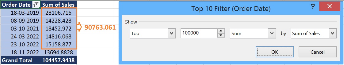
    • To filter by sum, select Sum.
  4. In the fourth box, select a Values field.

Top 10 Items dialogbox in a Pivot Table

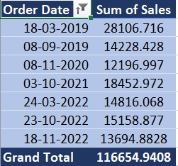
For below result, set the number as 5 in 2nd box in the Top 10 Filter dialog box,)
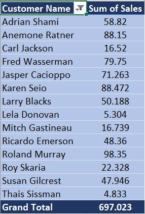
Then only the top 5 orders are now visible because of we filled 5 in the second box.

Top 10 Filter Result

2. Sorting Data
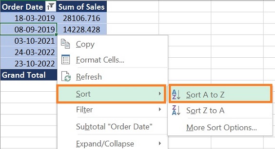
  1. To sort the amounts in Ascending or descending order, right-click on one of the amounts, and click Sort.
  2. Then click Sort Largest to Smallest for descending and Sort Smallest to Largest for ascending order.Pivot Table - Sort Largest to Smallest
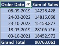
  3. To sort the date in ascending or descending order, right-click on one of the amounts, and click Sort.
  4. Then click Sort A to Z for ascending and Sort Z to A for descending.Pivot Table - Sort A to Z
3. Modify a Top 10 Filter

After you add a Top 10 Filter, you can change it, to show a different result.

  1. In the Pivot Table, click the drop-down arrow in the Order Date field heading.
  2. In the pop-up menu, click Value Filters, then click Top 10.
  3. In the Top 10 Filter dialog box, change the number of Items to 5 or 6 or whatever you want.
  4. Click OK, to close the Top 10 Filter dialog box, and apply the Value Filter.

The results change, to show only the 2 order dates with the highest sales amounts.

4. Filter a Pivot Table for Bottom 10 Items

The Top 10 filter helps you to find the highest amounts, but sometimes you need to find the lowest amounts, to focus on those. Even though the filter is named “Top 10”, you can use it to find the bottom (N) amounts too.

To see only the Bottom (N) order, follow the same steps as followed above for top 10 items and just change the first column option from Top to Bottom.

Filter a Pivot Table for Bottom 10 Items

The results will show only the (N) order dates with the lowest sales amounts.

5. Clear the Field Filters

When you’ve finished analyzing the filtered data, you can clear the Filters, to see all the data again.

  1. In the pivot table, click the drop-down arrow in the OrderDate field heading.
  2. Click Clear Filter From OrderDate Field, to remove the filter criteria, and show all the data.
Clear the Field Filters in pivot table

2. Filter Top or Bottom Items that make up a Specified Percent of the Value

You can use the top 10 filters to get a list of the top 5% (or 20,30%…..etc.) of items by value.
Suppose you want to get the list of orders that make up 5% of the total sales then,

  • Click the drop-down arrow in the Order Date.
  • In the pop-up menu, click Value Filters, then click Top 10.
  • In the Top 10 Filter dialog box, set the columns as below then
  • Click OK, to close the Top 10 Filter dialog box, and apply the Value Filter
Filter Top or Bottom Items that make up a Specified Percent of the Value

This will give you a filtered list of orders that makes up 5% (Least) of the total sales.

Filter Top or Bottom Items that make up a Specified Percent of the Value Result

3. Filter Top or Bottom Items that make up a Specified Value Sum

Another way to use the Top 10 Value Filter is to find the items that make up a specific sum. For example, from the order dates with the highest sales amounts, which order dates would combine to total at least 1,00,000 in sales?
To see this, follow these steps:

  1. In the Pivot Table, click the drop-down arrow in the OrderDate.
  2. In the pop-up menu, click Value Filters, then click Top 10.
  3. In the Top 10 Filter dialog box, change the settings as below

The results will show only the 6 top order dates because their combined sales are at least 1,00,000.

As you can see in the pivot table shown below, the top 5 order dates only total 90,763.061, so the 6th top order date is also included in the Value Filter results to achieve a 1,00,000 minimum.

4. Filter Items based on value (Criteria/Condition)

Filtering particular items based on values in a pivot table in Excel is a useful tactic to focus on specific data that meets certain criteria.
You can use the “Value Filters” or “Label Filters” options in the pivot table to filter items based on values. Follow the steps below:

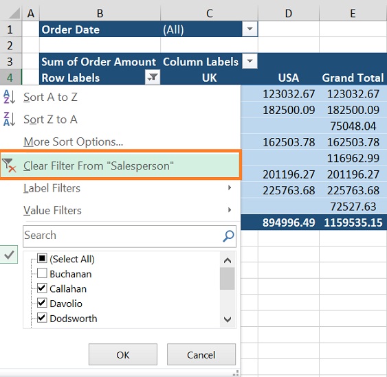
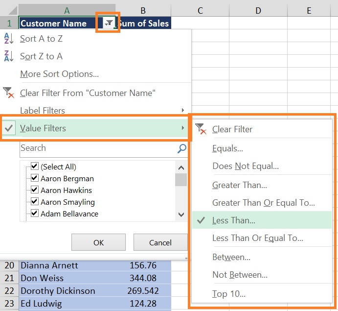
  • Click on the drop-down arrow beside the field you want to filter in the Rows or Columns area of the pivot table.
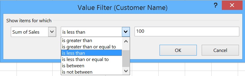
  • Choose “Value Filters” then select appropriate filter options, such as “Equals,” “Greater Than,” “Less Than,” etc.Filter Items based on value in pivot table
  • Once you’ve selected the filter option, you’ll be prompted to specify filter criteria and criteria value.
    • Select the field name (Column) on which you want to filter in 1st dropdown option
    • Select criteria, whatever you want to apply in 2nd dropdown option
    • Enter the desired value or range, and click OK.Filter Items based on value condition in pivot table
  • The pivot table will now display only the items that meet your specified value filter criteria.

Similarly, there are numerous other conditions that you can use such like equal to, does not equal to, less than, less than Or equal to,  between, not between, etc.

Also, keep in mind that filtering items based on values in a pivot table is a powerful tool for data analysis, but if your filtering requirements are complex or require more advanced calculations, you might need to use Excel’s formulas or even consider using Excel’s Power Query or Power Pivot features.

Leave a Comment