Label Filters In Pivot Table

Label filters is an in-built feature of Pivot Table. You can use the feature of the Label Filters in the Pivot Table to filter data based on specific criteria/conditions. It allows you to select specific items based on text values in the rows/columns level filter of the pivot table.

Contents

It works when you have a huge list and you want to filter specific items based on their name/text and it will display only the data that meets certain conditions, making it easier to analyze and summarize your data.

How to use Label Filters in a Pivot Table, Follow the steps below:

Add Fields to use Label Filters

Drag the field you want to use for analysis to the either in row or column areas in the PivotTable Fields list.

Apply Label Filter

Click on the drop-down arrow beside the field you want to filter in the Rows or Columns area of the pivot table.
Choose “Label Filters”
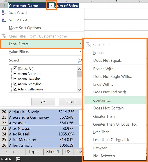
Now you will see many filter options as below:
- Equals: It is used to filter data that are equal to a specific value or Text with an exact match.
- Does Not Equal: It is used to filter data that do not equal a specific value or text you mention. It is exactly the opposite of the above “Equals” filter.
- Begins With: It is used to filter data that begins with a specific text you mention.
- Does Not Begins With: It is used to filter data that do not begin with a specific text you mention. It is exactly the opposite of the above “Begins With” filter.
- Ends With: It is used to filter data that end with a specific text you mention.
- Does Not Ends With: It is used to filter data that do not end with a specific text you mention. It is exactly the opposite of the above “Ends With” filter.
- Contains: It is used to filter data that contain a specific text either in the middle, beginning, or end.
- Does Not Contain: It is used to filter data that do not contain a specific text. It is exactly the opposite of the above “Contains” filter.
- Greater Than: This is a value filter used to filter data greater than a specified number you mention.
- Greater Than or Equal To: This is a value filter and it is used to filter data that is greater than or equal to a specified number you mention.
- Less Than: This is a value filter and it is used to filter data that is less than a specified number.
- Less Than or Equal To: This is a value filter and it is used to filter data that is less than or equal to a specified number.
- Between: It is used when you want to apply a filter between ranges. This means values that fall within a specified range you mention.
- Not Between: Filter for values that do not fall within a specified range. It is exactly the opposite of the above “Between” filter.

Set and Apply the Label Filters Criteria

Depending on the filter option you chose, you’ll need to specify the criteria. For example, if you choose “Equals,” you’ll enter the specific value you want to filter by. If you choose “Between,” you’ll enter a range of values.
Then click OK to apply the filter.

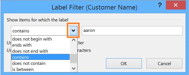
The pivot table will now display only the items that meet the label filter criteria. Here “aaron” is set as the “Contains” criteria, means if “aaron” available in customer name whether in first or last, will filter and display as result as shown below.

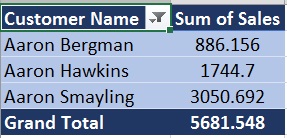
Label filters in pivot table are particularly useful when you want to focus on specific text values within your data without performing mathematical calculations.

Clear the Filter

To remove the Label filter in pivot table and display all data again, you can either go back to the filter drop-down and select “Clear Filter,” or you can uncheck the filter criteria you applied.

Multiple Filters on a Pivot Field

There are some facts about applying multiple filter types in a pivot table at a time.

By default, you can use only one filter type at a time in each pivot field.
If you try to use another type of filter, the first pivot filter will automatically be removed.
Excel doesn’t give any warning message that the first filter is removed.

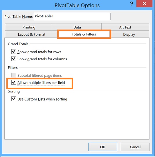
But by setting in the pivot table option, multiple filter types at a time on a field can be applied. Follow the below steps:

Right-click on a cell in the pivot table, Then click “Pivot Table Options”.
Or
Go to Analyze tab in PivotTable Tools menu then select Options in PivotTable group tools.
In the Pivot Table Options dialog box, click on the “Totals & Filters” tab
In the Filters section, add a check mark to ‘Allow multiple filters per field.’
Click the OK.

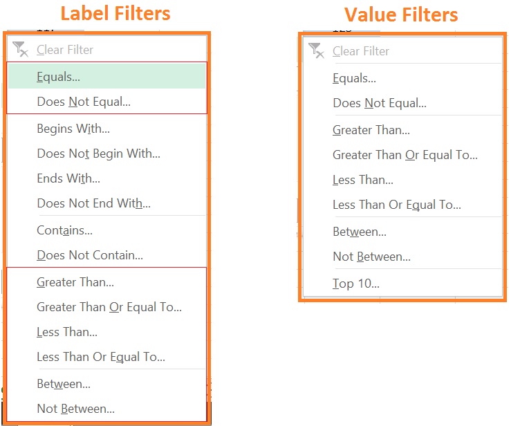
Difference between Label Filters & Value Filters

Label & value filters are in-built filters in a pivot table. The main difference between both is that:

If you filter your data based on number i.e. value, then you will have to use Value Filters and.
If you filter your data based on Text then you will have to use Label Filters. But some value filters will also show up in this filter but don’t be confused about the working of those filters as mentioned above.

Something interesting, when you filter data using Value/Label filters, is that some options are common except the Top 10 filter which belongs in Value Filters.

Related Topics